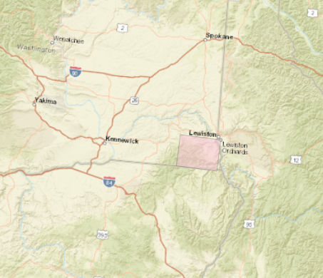
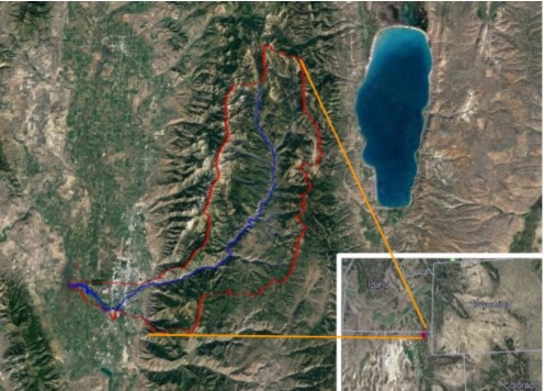
Introduction: Regional Geography, Geology, and Climate
The Payette River drains the southern portion of Valley County in central Idaho. The catchment shares divides with the Salmon River to the North and East, the Boise River to the Southeast, and Cottonwood Creek to the West. The north and south forks confluence in Banks, Idaho (850 m) and continue flowing south for 20 km to the town of Horseshoe Bend (800 m). In Horseshoe Bend, the watercourse turns west and cuts through a final canyon before entering a broad valley between Emmett, Id and Ontario, Ore. The Payette River then confluences with the Snake River upstream of Hells Canyon on the Oregon/Idaho Border (650 m). The Lower Payette Valley is a region of extensive agricultural development. For this project, we will specifically focus on the North Fork of the Payette River.
Figure 1: Location map of NF Payette drainage
Drainage networks in the region are structurally forced by geology associated with Cretaceous accreted terranes and the Idaho Suture Zone to the West. To the East, underlying geology consists of Pre-Cambrian metamorphic and Cretaceous intrusive igneous formations. Drainage networks to the east are more dendritic. The watershed can be generally divided into three regions: alpine headwaters, Long Valley, and the lower canyon. Alpine headwaters, mostly to the north of McCall and the eastern margin of the watershed account for most of the sediment and snowmelt supply. Long Valley, between McCall and the Cabarton Road bridge, is a low-relief valley formed by normal faulting. Payette Lake to the north is a natural glacial lake serving as a contemporary sink. Cascade Reservoir in the middle of the valley is a 646,000 acre-foot impoundment formed in 1948 by a 70-ft dam (USBR). The lower canyon between Cabarton Bridge and Banks is a mostly confined reach with dramatically increased valley slope and anthropogenic impacts associated with highway and railroad construction.
Figure 2: Confinement in lower canyon through highway and railroad construction
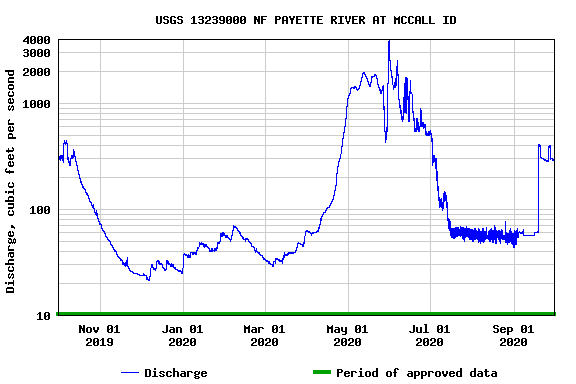
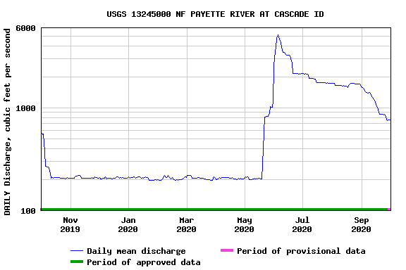
The total catchment area is 2585 square kilometers and the perennial stream length is 65 kilometers. The North Fork Payette River is a snow-dominated intermountain catchment where annual peak flows are driven by snowmelt. A majority of annual precipitation falls as snow and July and August are very warm, dry months. The flow is subject to minor imposed controls below Payette Lake, but the USGS gaging station near McCall reflects mostly natural flows. Cascade Reservoir, as the largest reservoir in the Payette and Boise watersheds, is operated to satisfy summer irrigation objectives downstream and attenuates the natural hydrograph accordingly.
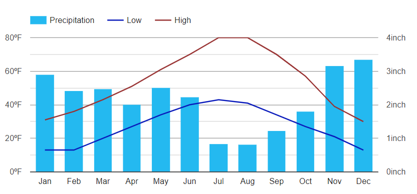
Figure 3: Monthly climate averages for McCall, Idaho (NOAA)
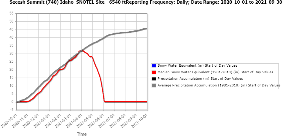
Figure 4: Average annual precipitation patterns at Secesh Summit SNOTEL site (USDA)
For the purposes of this report, we will focus on sites at the downstream end of the catchment where they are affected by anthropogenic factors such as valley confinement and and flow impairment/sediment blockages.
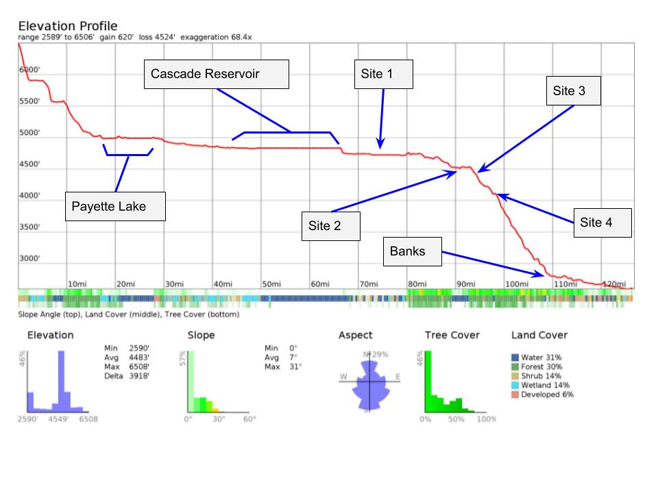
Figure 6: longitudinal profile of the NF Payette, extending past the SF confluence to Horseshoe Bend, ID
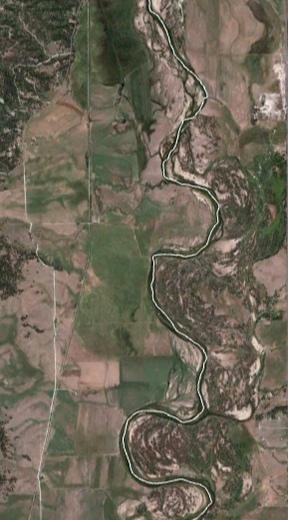
Site 1: Cascade Valley (unconfined)
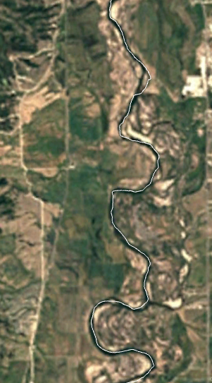
The first site to consider is within the broad valley just downstream (south) of the town of Cascade. The river flows through a sheet of glacial outwash sediments with expansive terraces along both sides of the valley. In some places, the channel is somewhat confined by the terraces, but high flows have had a tendency to rework confining slopes and promote lateral migration of the channel. Local landowners have made some efforts to stabilize banks, such as tree revetment projects. Comparing satellite imagery from 1985 to 2019 indicates that very little channel migration has occurred, largely due to flow impairments.
, The river bed material consists mostly of sand and small gravels. The uncommon occurrence of pea gravel is made possible in this case by the large crystal sizes found in upstream source materials and the glacial origins of much material in the valley. The watercourse distance through the reach is 15.0 km while the valley centerline length is 10.0 km. The sinuousity of the channel is 1.5. Average meander amplitude is 400 m and wavelength is approximately 1.5 km.
This reach features many prograding point bars with ridge and swale complexes highlighted by vegetation patterns. The elimination of high flow events has also allowed for vegetated islands to remain in place. Several of the larger pointbars also feature high-flow channels connecting to the mainstem at both ends of the feature. Other high-flow areas are disconnected, forming backswamps. Along cutbanks, collapses of soil undercuts often brings lodgepole pines and other coniferous trees into the water. No boulders exist in the channel and the river is too wide for trees to broach the whole channel, so they are generally swept downstream by high flow events unless anchored to shore by their root balls. Within the channel many diagonal bars split the flow. Many of these features have started to harbor perennial vegetation, which is enabled by the hydrological attenuation of Cascade Dam. The length of many of these diagonal bars ranges from 180 m to 400 m. In many cases, the avulsion channels on the inside of the diagonal bars have developed their own depositional architecture with smaller point bars extending 50-100 meters. It is possible that the general watercourse and larger wavelength meander structure of the river was developed under a prior hydrologic regime and the river is now developing a new set of smaller structures driven by a change in flux boundary conditions overprinted on an ancestral riverscape. Site 2 - Smith's Ferry (partly confined, planform controlled)
Downstream of the valley, the NF Payette enters a narrow canyon. The canyon widens for a short section known as Smith's Ferry. Within this reach, the river is partially confined with a confinement ratio of 0.65. The extent of modern floodplains are again difficult to ascertain, as the upstream flow controls have reduced the magnitude of high-flow events. The bed material is mostly sand with some finer material on floodplains. Many mid-channel bars have vegetation, suggesting a decrease in high-flow events. High flow channels on the backside of point bars and mid-bar headcuts and chutes are also common. The upstream end of the reach features an expansion bar, as the channel width quickly widens from 17 m to 128 m.
Site 3 - Lower Canyon (fully confined)
The low slope of reach 2 is partially driven by tectonic influences on the base level just downstream. The same tectonic influences have created a hinge point in the longitudinal profile of the watercourse. Below this hinge point, channel slope increases significantly (average slope: 0.032 compared to 0.002.) This dramatic increase in absolute stream power is amplified in specific stream power by a decrease in channel width (11-15 m). The narrowing channel is partially a product of v-shaped valley incision through bedrock, but also enhanced through anthropogenic confinement. A railroad on one bank and a major state highway (ID 55) on the other have further narrowed the channel. Bed material is almost entirely large boulders. Sand entering the reach is readily conveyed downstream with virtually no deposition. A few small bank-attached sand pockets exist in back eddies, but are submerged at low flows.
With no floodplain pockets and minimal bank-attached features, the reach is fully confined on both banks throughout its length. We can focus geomorphic interpretation on the longitudinal concavity of the bed, as interpreted through hydraulic behavior on the surface. Units are defined as runs, rapids, and pools. All pool-rapid transitions involve a convex crest, but those features are only identified when they have a longitudinal footprint greater than 20 meters. The reach generally features an alternating sequence of runs and rapids (distinguished by bed material and hydraulic energy) separated by short pools. 2.3 kilometers of the 4.2 kilometer reach constitute rapids. The longest single rapid unit extends 1.2 km. Kayakers sometimes refer to this as phenomenon as "full-on rowdy class V." Site 4 - Big Eddy (mostly confined, floodplain pockets)
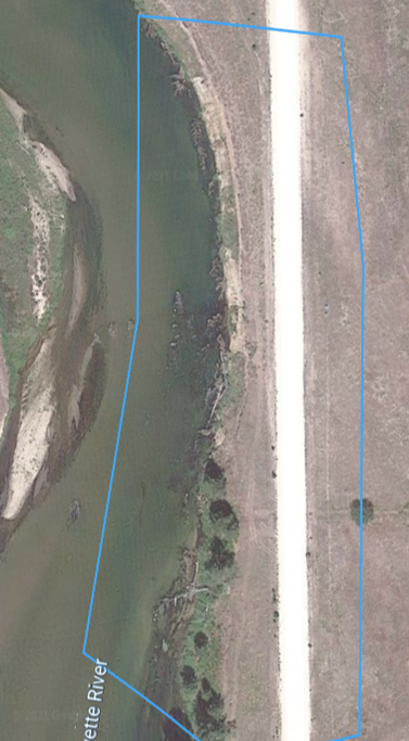
The final reach is a short section within the 25 km lower canyon where the valley slope reduces to 0.003 and depositional units are present. In the "Big Eddy" reach, floodplains also exist but the channel abuts at least one margin for 85% of the reach length. The bed material is mostly sand, though some fluvial bank-attached cobble bars occur at the upper end of the reach. The middle of the reach is dominated by a diagonal bar. The avulsion occurs on the road side of the channel and it is possible that the avulsion is further enhanced by the confining margin of highway rip rap.
Overview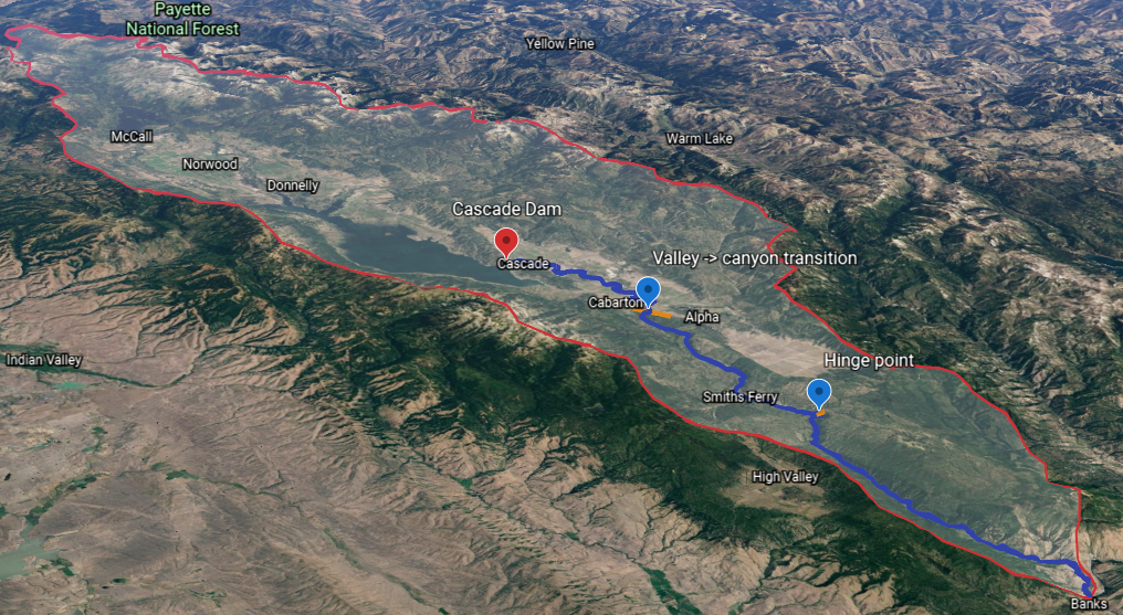
Figure 12: Oblique view of the NF Payette watershed
As shown in Figure 6, the lower canyon of the NF Payette represents a significant knick zone with a greatly steepened valley slope from the upstream reaches. With flow impairment associated with Cascade Reservoir, the capacity of the river to transport sediment is limited by the gentle slope of the upstream valley. Any sediment that can be moved through the valley will be easily conveyed through the canyon, though the canyon is unlikely to be incised quickly under the contemporary hydrologic regime. The North Fork Payette is a riverscape recently redefined by changed boundary conditions and superimposed on a landscape shaped by a previous climate and tectonic setting.
References
https://digitalatlas.cose.isu.edu/counties/valley/geomap.htm
caltopo google earth https://www.usbr.gov/projects/index.php?id=10 https://www.usclimatedata.com/climate/mccall/idaho/united-states/usid0156
0 Comments
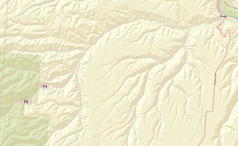
The Geomorphic Unit Toolkit (GUT) is a plug-in for ESRI ArcMap developed by Utah State University in 2017. It provides an extensive set of tools for mapping and analyzing surveys of fluvial channels. In this exercise, we are not running any parts of the toolkit, but simply looking at some of the analyses of surveyed DEMs and identifying geomorphic structures. The area of study is the North Fork of Asotin Creek in Southeast Washington, USA. The toolkit uses a taxonomic framework developed by Wheaton et. al. (2015) to identify units by their position, form, and unit type. LocationAsotin Creek flows north and east into the Snake River. The canyons are cut through the Columbia River Flood Basalt geologic province of eastern Washington. Site F6 is located upstream of F4 and both are along the North Fork of Asotin Creek. Neither site received restoration modifications during the study period.
Interpretations - Site F42.1: Qualitatively describe the in-channel geomorphology of this reach. The channel is relatively straight with a mid-channel thalweg. Small pool concavities are scattered throughout the stretch with concave troughs separating them. Some channel changes and unit shifts have occurred between 2011 and 2017, but nothing that substantially changes the character of the reaches. 2.2: Choose at least two survey years at this site to consider the temporal variability of morphology at this site. Which survey years are they and why did you choose them? I have somewhat arbitrarily chosen 2013 and 2017 2.3: What Tier 2 Forms are present in each year? Do they differ? In both years, we see bank attached convexities and mid-channel troughs and pools. Planar structures are generally limited to the margins. The positioning and occurrence of features is generally consistent between the two years, though a mid-channel convexity develops at the upstream end of the reach as shown in figure 2. 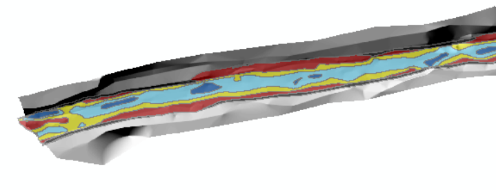 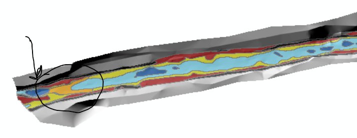 figure 2: upstream end of reach in 2013 (above) and 2017 (below) with new convexity circled 2.4: Do any of the Tier 2 Forms dominate the assemblage or is it fairly mixed? Is this true through time?
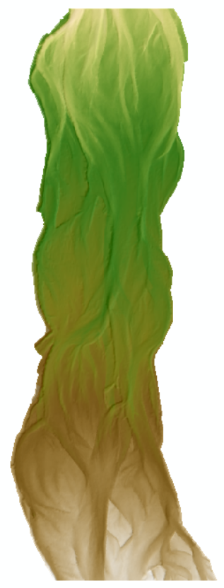
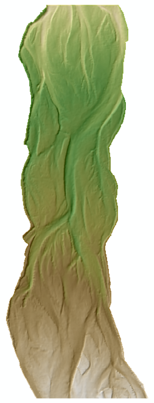
Pools and troughs are dominant in both years. 2.5: What Tier 3 Geomorphic Units are present in each year? 2.6: Zoom in to 2 to 5 x bankfull width portion of the reach and look at the arrangement of geomorphic units. Is it coherent? Does it make sense based on what you have learned so far? 2.7: How well does GUT appear to be doing in each year at discriminating the in channel geomorphic units? Point out any weaknesses or concerns you might have. 2.7: Identify in one of your surveys for this reach a distinctive pool, bar and planar feature. For all three identify all five attributes from the fluvial taxonomy (i.e., Table 6), then use those to identify the tier 3 name from Table 7 or 8 (this may differ than what GUT output is because it is not as resolved) and explain which attribute(s) were key for discriminating that unit from other units. In unconfined settings, rivers can adjust the geometry of their channels in all directions. Channels can shift laterally or widen through bank erosion and constrict through bar development. The elevation of the riverbed surface can adjust through aggradation or progradation. Examples of all four processes will be observed and described below. This lab was completed using ArcMap 10.7 (ESRI) and GCD (Riverscapes Consortium) software. High-resolution DEM surfaces were provided of the reach area from five consecutive year (2003-2007). The GCD software streamlines a workflow to consider a threshold of certainty (80% for our purposes) and report all areas where the elevation increased or decreased and by how much. The GCD software then produces summative statistics to determine the area and volume of bed aggradation or degradation and the net change in volume between any two surfaces. I chose to examine 2-year intervals: the first from 2003 to 2005 and again from 2005 to 2007. Elevation surfaces for each survey are show below with effectively equal color ramps:
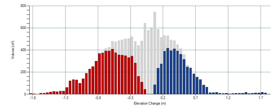
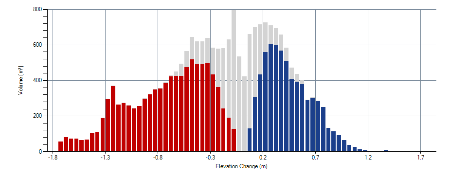
In a change detection, each pixel is evaluated for positive or negative elevation change and those surpassing a 80% confidence threshold are reported. The volume of material added or removed from the bed can be expressed by frequency histograms as below:
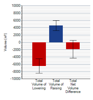
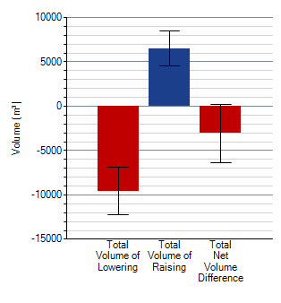
Looking at the histograms suggests both periods were degradational, but total changes throughout the study area are also cleanly reported by GCD as bar plots:
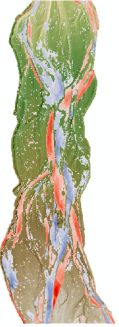
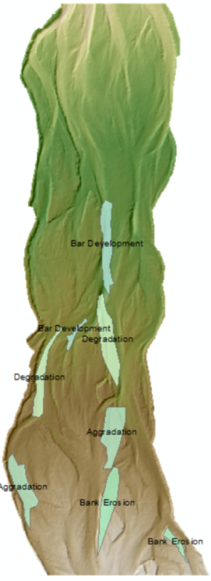
These plots illuminate that the reach was in net degradation throughout both epochs I considered. Note the difference in vertical scales: There was more total erosion and deposition of sediment in the later timeframe. By visually comparing the topography to the zones of aggradation/degradation, it is possible to separate some of the raising into aggradation or bar development based on whether the channel expands laterally or not. Likewise, lowering can be separated into degradation or bank erosion. The images below show where I identified each of the four mechanisms of channel reconfiguration. All images are with the 2005 base DEM. Aggradation and degradation occur when the area is part of the channel both before and after.
The GCD software additionally allows for budget segregation. The polygons drawn and labeled above can be analyzed individually or as groups to determine the areal extents or total volume of material deposition or removal. For example, the total area of bank erosion as I've identified was 1425 square meters, the area of bar development was 1298 sq. m. The total volume of bar development, however, was approximately half that of bank erosion.
On February 8, 2021, we convened in small groups to make experimental observations of fluvial process in a simulated flume. The flume consisted of a large aluminum tray containing color-coded engineered experimental sediment and a water pump set up to continuously circulate water. The flow rate of the flume could be adjusted digitally with pump controls
The outlet of the flume was a vertical cylindrical pipe which could be slid up and down to adjust the base level of the system. Adjusting the base level would in turn adjust slope, although slope could also be established by changing the sinuosity and therefore the length of the channel. 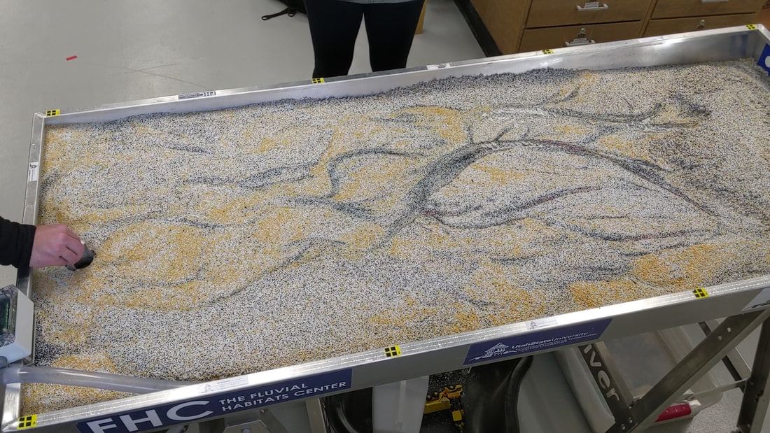
Adjusting the outlet elevation. Photo: Joe Wheaton
Several geomorphic processes were simulated in the flume. Bed erosion occurs when sediment is scoured from the bottom of the channel. Particles in motion represent transport. Bank erosion refers to sediment on the lateral margins of the channel breaking loose and moving into the flow. Deposition occurs where the flow slows down locally and particles cease their downstream travel.
The coloration of grains illustrate grain sorting. The largest grains are yellow, followed by white, black, and red. The yellow grains are generally more resistant to transport and we see much more entrainment of white and black grains. The red sediment is counterintuitively stable in fast currents, largely because it is small enough to embed in interstitial spaces and be protected from flow forces. Most channel forms involved braided systems with multiple channels. Point bars could be seen to be cut off through avulsion and chute dissection occurred via headwards erosion of small channels within bars as seen in the video below.
Individual meander bends were possible for us to observe in the flume, but no conditions resulted in a stable single-threaded meandering channel. This is due to the lack of cohesion in the environment, which is necessary to adequately stabilize the banks.
Using the adjustable pumping rate, we simulated a set of floods. In the small flood event, increased flow created a surge over the floodplain and short-term channel incision on the flood plain. During the recession limb of the event, the channels were mostly filled back in by aggradation and the flow returned to the original channel.
In a larger flood event, by both duration and magnitude, the surge cut through the floodplain and dramatically altered the architecture of the channel. Again, the sedimentation patterns during the recession limb tended to establish the layout of the resulting channel.
At different flow stages, we observed bankfull flows, where significant transport and braiding restructuring occurred as well as base flow when very little transport occurred. Overbank flows were required to re-route the stream, though bankfull flows could cause small adjustments to the course. Due to the very high permeability of the sediment in the flume, there was significant hyporheic flow which was a main driver of channel incision in addition to supporting entrainment of sediment flows rising up from beneath the bed can exert and upward force on grains.)
Photo #1 below shows the complexity of flow direction and speed within a short but steep drop. The light blue line (F) labels a flow seam where a variety of flow directions converge and fold over each other resulting in a subducting flow. This photo shows a chute.
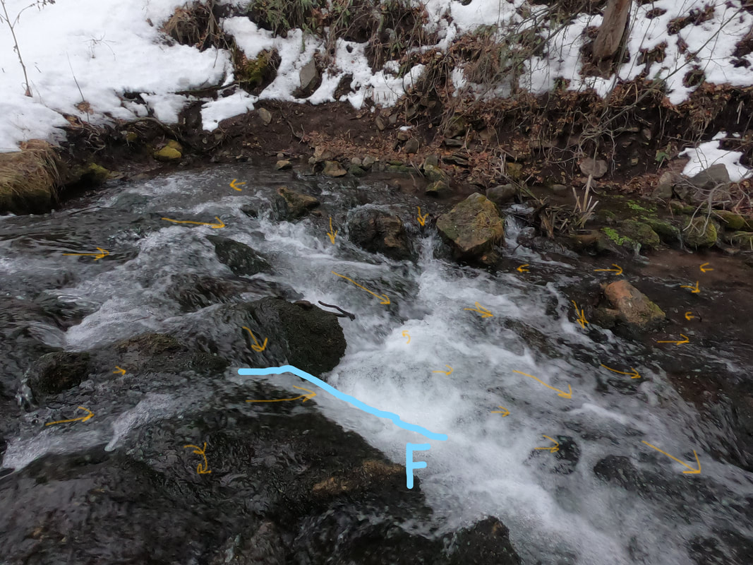
Photo 1
Photo #2 below highlights several flow features.
Photo 2
Photo #3 is taken closer to a boulder and more closely illustrates the divergent flow on the upstream surface and the zone of reattachment on the downstream end.
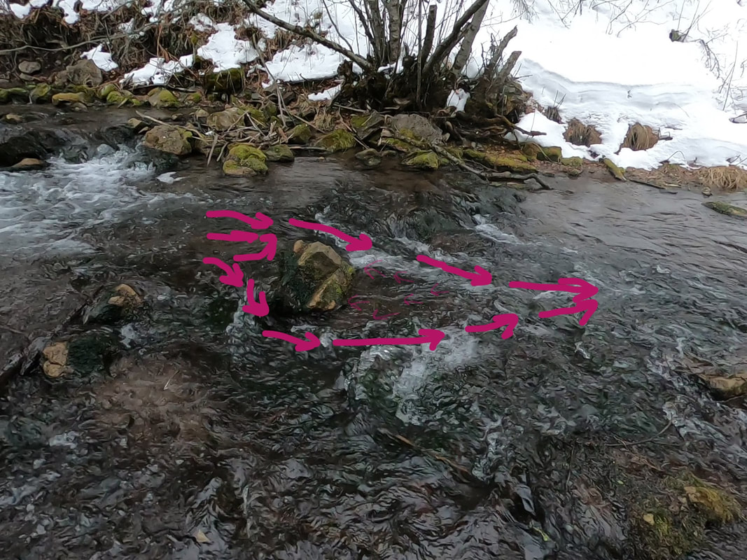
Photo 3
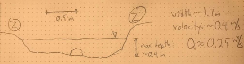
An approximate cross section was drawn according to the line shown in photo #3. Depth and width were estimated without wading. The velocity was estimated using a piece of flotsam that traveled approximately 1 m in 2.5 s. This produced the discharge estimate shown below, but this estimate is likely high as the measured velocity is probably above average for the cross section.
The image and video below (Photo #4) illustrate a hydraulic jump. Many hydraulic jumps exist in boulder drops, but the phenomenon is perhaps most clear on this small example. Progressing from the upstream end, the flow is characterized as subcritical flow (A) until it passes over a submerged rock and transitions to supercritical flow (B). The hydraulic jump is indicated by air entrainment and backwash in the flow (C) and produces an aerated and elevate water surface downstream of the jump (D)
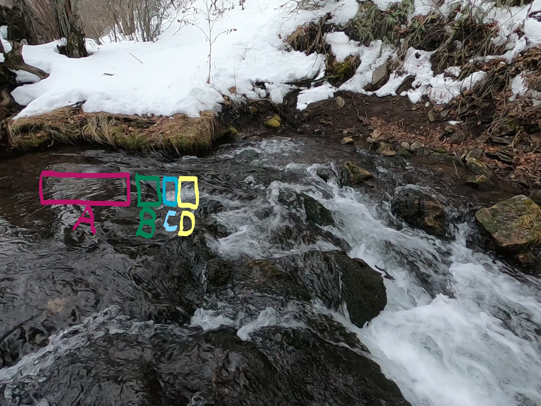
Photo 4
Hydrology is the study of water as it moves through the water cycle. Primarily, water can exist as atmospheric moisture, cellular water, surface water, or groundwater. The mechanisms through which water moves between these storages are defined by a variety of critical processes. Many of these processes can be observed on small scales close to home. Below is my bingo board where I will attempt to capture as many processes as possible throughout the semester.
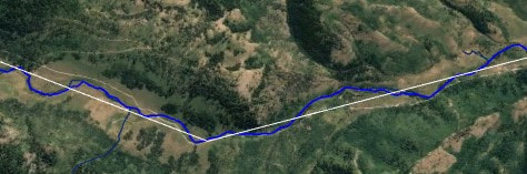
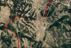
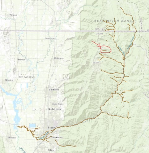
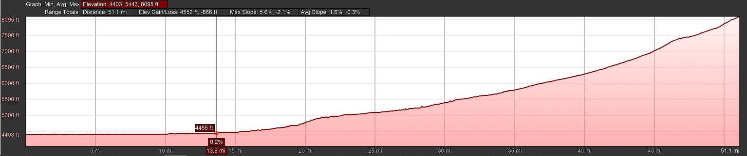 The Logan River descends from a valley elevation of 8,087 ft amsl to its current base level control of Cutler Reservoir at 4,408 ft over the course of 51 miles (82 km). During the Pleistocene, the base level was controlled by Lake Bonneville at an elevation of approximately 5,100 ft. (DeGrey, et. al. 2021) The concavity of the mainstem of the Logan can be calculated using the equation provided on page 32 of Fryirs & Brierly, 2013. Calculations are provided below: 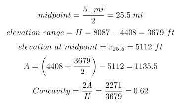 Fig. 3 - Concavity calculations of Logan catchment The profile of the Logan River is generally concave and well-graded, though two knickpoints can be easily identified. The first is just upstream of the river outlet into the valley. The second is near the headwaters. It is possible that the lower knick point is a product of changing base levels from the recession of Lake Bonneville while the upper knick point appears to coincide with the Klondike Fault and may have tectonic origins. 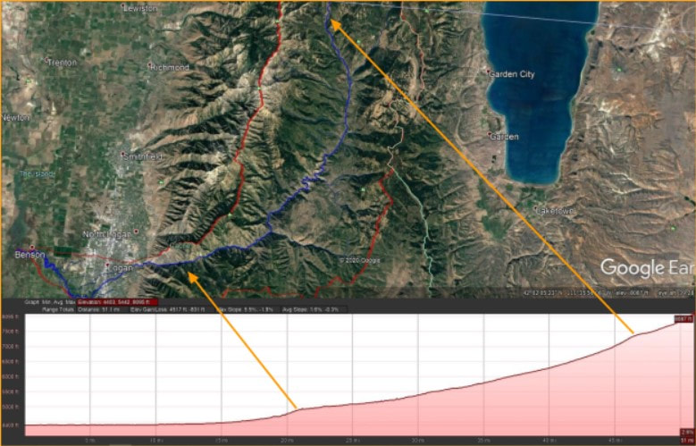
The highest point in the basin is Naomi Peak at 9979 ft (3042 m) expressing a total relief of 5571 ft (1698 m). The relief ratio is 0.05. It should be noted that the high point of the range is atypically located on the range front, about halfway between the headwaters and the outlet. Typical peak elevations near the headwaters are about 300 m lower than Naomi Peak.
Based on the provided stream network, the Hortonian stream orders can be calculated manually. At its mouth, Temple Fork is a 3rd order stream. Beaver Creek, with only one very small perennial tributary, is a 2nd-order stream. At the outlet into Cutler Reservoir, the Logan River is fourth-order. Other literature (Neilson, et. al. 2018) has identified the river as third order. This discrepancy aside, the Logan River network appears to obey the Hortonian laws of stream network composition. References Neilson, B. T., H. Tennant, Stout, T. L., Miller, M. P., Gabor, R. S., Jameel, Y., et. al. 2018, Stream centric methods for determining groundwater contributions in karst mountain watersheds. Water Resources Research, 54, 6708–6724. https://doi.org/10.1029/2018WR022664. DeGrey, L., M, Miller & P. Link, Lake Bonneville Flood, http://geology.isu.edu/Digital_Geology_Idaho/ Module14/mod14.htm, accessed 31 Jan. 2021 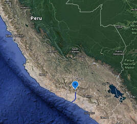 This assignment was to take 15 minutes to observe a river segment and write about it in the framework described in Chapter 1 of Fryirs & Brierly, 2012. I chose to use Google Earth to virtually visit the lower section of the Colca River in southwestern Peru. The location of the river segment I'm interested in is shown to the right. We will zoom in to the specific reach before considering local geomorphology in a regional context. I have selected the Colca River because some of the geomorphic units we can observe are rather large and are clearly visible from satellite imagery. All images below are screenshots from Google Earth: 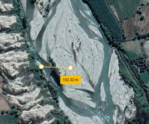 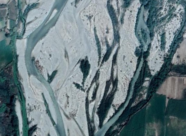 Based on the visibility of individual grains in these images, it appears to be a cobble-dominated riverbed. Vegetation patterns highlight abandoned channels or high-flow channels across mid-stream bars. Lateral bars are common, though the channel does periodically flow along the confining margins established by the elevated terraces. Many of these terraces are now cultivated and irrigated. In some cases, as shown below, the river character alternates between riffles and pools. Throughout this reach, the width of the valley bottom ranges from ~90-800m. The valley bottom is bounded on both sides by fluvial/alluvial terraces up to 60m high. 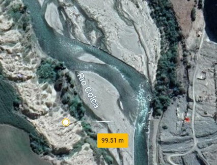 It is difficult to ascertain the existence of human-imposed controls. While development is obvious on both sides of the river, it seems to exist mostly on elevated terraces. High flows in the channel appear to be accommodated at the upstream end of the reach by a wide valley bottom and additional chute channels. At the lower end, it seems the river may have been stabilized to support construction of a bridge (just downstream of the image.) Where the road is visible in the last image, a seasonal tributary enters and impacts the channel geometry. In a slightly zoomed out view of the entire reach, we can see how the valley tapers and notice the settlement developed on a laterally contributing alluvial fan. 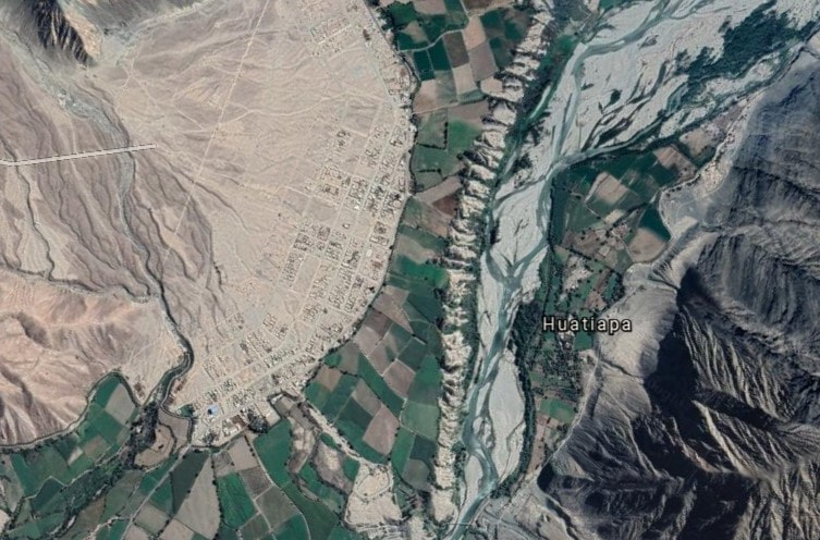 The volume of sediment developing the braided channel system and resiliency of the high terraces both suggest this is a transport-limited reach. In a larger context of the watershed, this is a dramatic shift in geomorphology. Just 13km upstream, the river is fully-confined and supply-limited, with very dramatic bedrock riverbeds in a high-gradient canyon. 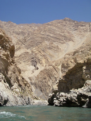 This transition represents a shift in hydrologic and tectonic setting. The Colca incises an extremely high-relief (>6,000 m) and tectonically active portion of the Andes Mountains. As the river approaches a base level at the Pacific Ocean and moves further from the center of uplift, the gradient of the channel decreases. What is likely more important than tectonic setting in driving this geomorphic transition is the confluence with a steep un-named tributary. Shown in the image below, the confluence with the steep tributary at Andamayo coincides with the development of terraces and establishes the combined system as transport-limited. 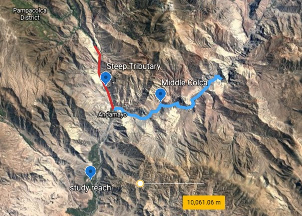 |