|
The objective of this exercise was to identify and analyze the home ranges of seven coyotes based on point data collected by tracking. In addition to identifying their core and general ranges, their actual use of different land cover types was analyzed and reported. 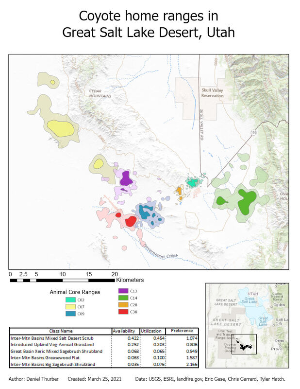 The workflow for this analysis drew upon previously-used tools such as point-polygon-raster conversions and interactions and raster reclassification. We also generated a point shapefile from a .csv file and used the kernel density geoprocessing tool to extend a probability surface to represent coyote ranges. The nature of this process explains why all of the ranges include multiple disconnected areas. The ranges shown represent areas where each animal is 50% (core range) and 95% (general range) likely be detected based on experimental data. Most significantly, this lab introduced us to automation of repetitive geoprocessing tasks using the ArcPy library in Python 3. We used a script previously developed by Chris Garrard and Tyler Hatch and applied it to our data directly through the geoprocessing toolbox. These scripts can also be executed independently in a Python console. Upon generating individual polygon files for each animal, the ranges and detection data were superimposed on land cover data to analyze what habitat was most available to the animals as a collective unit and where they were observed. The preference ratio refers to how frequently animals were observed in the given land cover compared to how much of that land cover was available. The 15 most available land cover types are reported below. 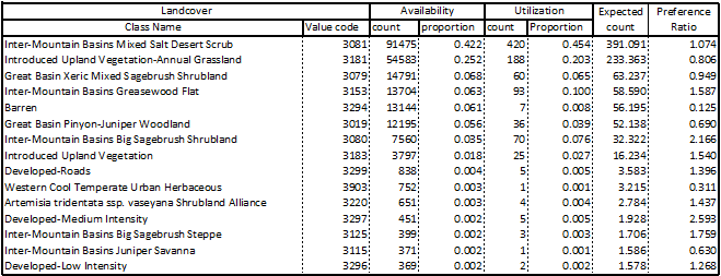 View a high-resolution PDF here.
0 Comments
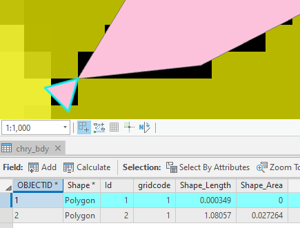
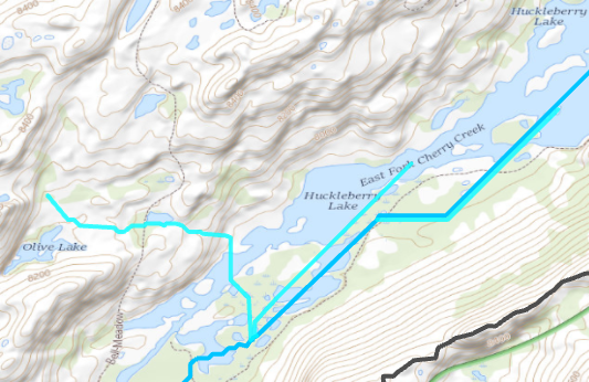
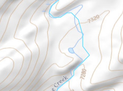
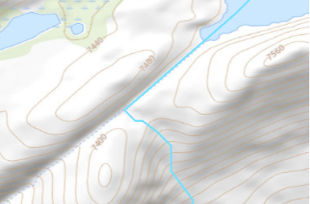
In this exercise, we delineated and characterized a stream network using ArcGIS Pro and included geoprocessing tools. Supporting the idea that a digital elevation model is the most useful application of raster data, all elements of this map were generated based on a 10m DEM from the USGS. I chose to analyze the watershed of Cherry Creek above the inflow to Cherry Reservoir in central California. We were advised to avoid lakes, which I dismissed out of curiosity to see how an abundance of lakes might impact the end result. Managing lakes put extra emphasis on the need to create a 'filled' DEM which is necessary to maintain continuity of the flow accumulator. I first processed the DEM into hillshade (shown), slope, flow direction, and flow accumulation layers. The flow accumulation layer is critical for placing the pour point, and ensuring it lies in the stream network. The pour point (just North of Cherry Lake) is used in conjunction with the flow direction raster to establish the watershed extent. Lastly, I used the flow accumulation raster to delineate the stream network and identify the stream order of each segment using the Strahler method. The outcome of the stream order calculation relies heavily on the threshold value used to classify minor watercourses as actual streams. In this case, I used the threshold of 0.8 sq km of contributing area. The threshold value establishes all points with greater than 8000 pixels of contributing area as part of the stream network. This was vetted by comparison to the US Topo ESRI base layer. This proved to be a reasonable estimation, though it is clearly not the same procedure used to generate the basemap as some "intermittent" streams were acknowledged in my analysis while "perennial" streams were missed. My analysis ignores aquifer composition, elevation, and land cover upstream, all of which can impact the potential for consistent water in a channel. 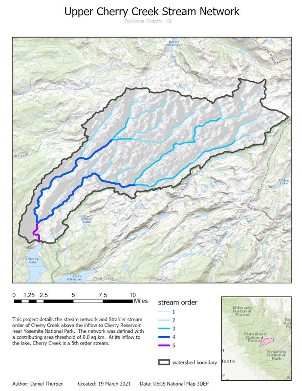 Total lengths of streams within the network are listed below. This generally follows the trend of decreasing length with increasing stream order, though the trend is not consistently geometric. 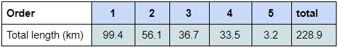 Figure 1: cumulative stream lengths for each class Throughout the geoprocessing, I noticed a handful of nuances that did not impact the integrity of the final results, but are worth noting. These oddities are described in figures 2-5 and are worth manually considering throughout the process.
As a final consideration, I wanted to compare the outcomes of this workflow to the automated watershed delineation tool provided by USGS Streamstats. This cloud-based program allows the user to identify a pour point and immediately delineate the pour point. The results were mostly consistent with a few notable exceptions. In the image below, the purple represents area included by both techniques. Pink was only included in the GIS analysis, blue was only included in the Streamstats analysis. The total areas of the two polygons were within 2%. Stream order calculations would not have been possible with Streamstats, although a great deal of climate data is automatically connected to the project. The Streamstats polygon appeared to be created using a DEM with ~100ft pixels, so the importance of raster resolution is evident once again. 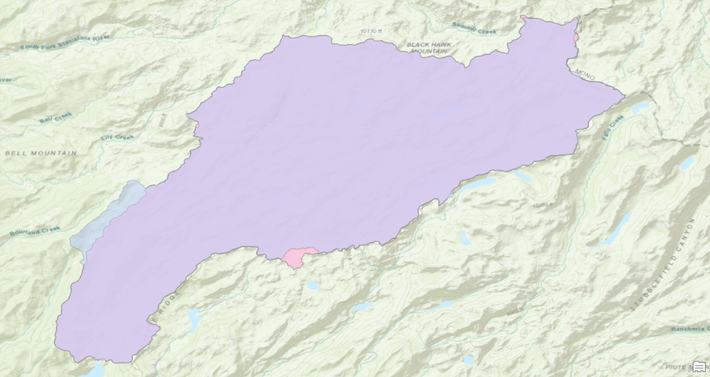 Fig. 6: Streamstats (blue) and ArcGIS Pro (pink) polygons of contributing area View a high resolution PDF here
The purpose of this exercise was to identify terrain suitable for spotted owl habitat in a canyon/plateau province of southeastern Utah. To accomplish this, I performed some basic DEM geoprocessing, condense rasters through reclassification, and calculate pixel values by combining several layers. Terrain was evaluated for suitability based on four criteria:
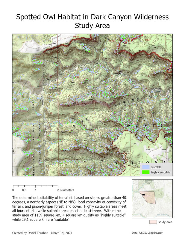 View a high-resolution PDF of the map here.
|
Advanced GISThis page is a repository of lab exercises produced for WATS 6920 - Advanced GIS Archives
April 2021
Categories |
 RSS Feed
